

A dashboard can be fast at 9:15 a.m. and frustratingly slow at 9:00 a.m. The SQL is the same. The underlying tables have not changed much. Yet the first click after a quiet period takes several seconds, while the next click feels instant. This is a common reason that teams misdiagnose performance: they compare one warm execution with one cold execution and assume the difference must be caused by the data model.
For Amazon Redshift users, the diagnosis changed in 2026. AWS introduced a query-compilation optimization that allows a new query to begin executing through a technique called composition while optimized query-specific code is prepared in the background. That is a meaningful platform improvement. It is not a guarantee that every dashboard will become fast, and it does not replace query design, capacity management or semantic modeling.
The practical executive question is no longer simply, “How do we warm the dashboard cache?” It is, “Which part of the user’s waiting time is compilation, which part is execution or queuing, and which part is outside the warehouse?” Answering that question prevents expensive fixes aimed at the wrong bottleneck.
The executive summary: what changed, and what did not
On March 18, 2026, AWS announced faster execution for new Redshift queries, reporting improvements of up to 7x for relevant dashboard and ETL workloads. AWS’s March 18, 2026 announcement explains that Redshift can start a new query using a lightweight composition of existing logic while query-specific optimized code is compiled in parallel. The improvement is automatic, at no additional feature charge, for supported provisioned clusters and Serverless workgroups. AWS’s later June 29, 2026 engineering explanation provides additional detail on the mechanism and its measured impact.
Three qualifications matter. First, “up to 7x” describes an observed upper-end result, not a contractual or typical improvement for your workload. Second, compilation is only one component of end-to-end dashboard latency. Third, the initial announcement’s maintenance-track rollout evolved: the announcement now specifies both maintenance tracks beginning with Redshift Patch 200. Check Redshift cluster-version notes and your environment rather than assuming an older patch has identical behavior.
The decision implication is straightforward: do not start a major warehouse migration or dashboard rewrite based only on historical first-run latency. Re-measure on a current supported Redshift version, then isolate the remaining causes.
What happens between a dashboard click and a rendered chart?
A BI interaction is a chain, not a single SQL statement. The user selects a filter or opens a report; the BI application evaluates its semantic model, generates one or more SQL requests, obtains a connection, and submits queries. Redshift admits those queries, plans and prepares them, reads or computes the required data, and returns results. The BI tool then transfers, aggregates or formats those results and draws the page. Authentication, network conditions and browser rendering can add delay.
A useful latency budget separates at least five intervals: BI application and connection overhead; warehouse queue time; query preparation and compilation; actual execution and data movement; and result transfer plus visualization. If the dashboard triggers twelve queries, the perceived delay depends on whether those requests run in parallel, wait on shared resources or depend on one another.
This is why “the SQL took 400 milliseconds” does not prove a dashboard should render in 400 milliseconds. It may be waiting on a slowest visual, an expensive semantic-model calculation, a queued query, a gateway or a large result payload. Treat the user-visible page load as the outcome metric and warehouse timings as diagnostic components.
Why first-run queries were historically slower
Redshift uses code generation to optimize execution. It can generate specialized code for a query and reuse compiled code for similar queries when available. Historically, a query shape that had not been compiled could incur a one-time compilation cost before efficient execution began. This was especially noticeable for otherwise short queries: adding two or three seconds of preparation to a 200-millisecond aggregation makes the first interaction feel dramatically slower.
A cold query is not necessarily a query against cold data. These are different concepts. Compiled-code reuse, result caching, operating-system or storage caching, and materialized-view refresh state can each influence performance. A dashboard that appears fast on repetition may benefit from one or several of them. Conversely, a new parameter combination may generate a distinct query shape even if the data is already in memory.
Consider a hypothetical revenue dashboard. Opening the report runs a filtered aggregation by region. Changing from “North America” to “Europe” may reuse a prepared shape or a cached result depending on the SQL and execution conditions. Adding a new grouping or switching to a different measure may produce a query that has never been compiled. The correct question is not whether the user has opened the dashboard before; it is which SQL and execution paths are actually being reused.

How the 2026 composition optimization works
The new approach checks whether suitable optimized compiled code is already available. When it is, Redshift can use that code. When it is not, composition assembles a lightweight execution path from existing logic so the query can begin without waiting for the entire query-specific compilation step. Optimized code is compiled concurrently for subsequent benefit. This removes much of the historical compilation delay from the critical path of new-query execution.
AWS reported that, among the small subset of query segments that previously missed its compilation cache, median compilation time in its analysis fell from 4.3 seconds to 170 milliseconds. That is a measurement of compilation time for that subset, not a promise that a complete dashboard will load 25.7 times faster. AWS also reported that more than 99% of queries across its fleet already used cached generated code before the change, an important reason why improvements vary by workload.
The likely winners are short, diverse, latency-sensitive queries: dashboards with many filter combinations, exploratory analysis, parameterized reports, generated SQL and some ETL orchestration patterns. A heavy query that scans large volumes, spills intermediate data or waits behind competing jobs will still spend time on those activities. Composition makes preparation less likely to dominate; it does not make expensive work disappear.
Where executives should expect the most visible benefit
1. Interactive executive dashboards.
A leadership dashboard may be opened by many people at different times, with distinct filters, date windows and access rules. When first-use query shapes are common, reducing preparation overhead can improve the perceived responsiveness of new interactions. The benefit should be measured at the visual and page levels, not inferred from the platform announcement.
2. Self-service exploration.
Analysts frequently create combinations of dimensions and measures that have not been executed before. A faster first response makes exploration less disruptive, but high-cardinality joins and poorly defined metrics can still produce expensive SQL. Teams should distinguish faster startup from a genuinely scalable semantic model.
3. Embedded analytics and customer-facing products.
A customer changing filters expects consistent response times. For these experiences, p95 or p99 latency and concurrency are often more important than a favorable average. Compilation improvements may reduce one source of variability, but capacity isolation, workload management and application caching remain relevant.
4. Scheduled transformations and ETL.
Repeated scheduled SQL can already benefit from compilation reuse, while generated or changing SQL may see more improvement. End-to-end pipeline duration also includes ingestion, dependency waits, writes, retries and data-quality checks. Do not report a query startup gain as an equivalent reduction in time-to-data.

The four bottlenecks the compilation update does not solve
1. Queries that perform too much work
If a dashboard scans a large fact table for every visual, joins raw event records at the wrong grain or calculates the same complex metric repeatedly, execution cost remains. Inspect scan volumes, join patterns, skew, intermediate results and the physical layout. Consider pre-aggregated marts, appropriate materialized views, selective filters and a stable semantic layer. Avoid assuming every problem needs another cache; sometimes the correct solution is a better data product.
2. Queueing and compute contention
A query can be ready to run but wait because resources are busy. Large ETL jobs, exports and interactive dashboards may compete for compute, especially at peak hours. Review workload management, concurrency, query priorities and whether workload isolation is justified. Faster compilation does not increase available compute or guarantee fair scheduling. Measure queue time independently from execution time.
3. BI-generated SQL and excessive visual requests
A report with twenty tiles can generate dozens of warehouse queries. Some are redundant; some use complex calculated fields; others return far more rows than the visual needs. Review how the BI tool folds transformations, applies row-level security and batches requests. Simplifying the report or its semantic model may deliver more value than tuning one isolated SQL statement. Actiknow’s custom BI dashboard development offering is relevant to this design layer, including data integration, dashboard development and testing.
4. Freshness, networking and application rendering
A dashboard can appear slow because it waits for a refresh, an API, a gateway, or the browser. A materialized view that is stale may need work before it is useful; a wide result set may be expensive to transmit; and complex visual rendering can dominate after SQL completes. Build traces across the whole request path. Warehouse-only tuning will not fix a slow client application.
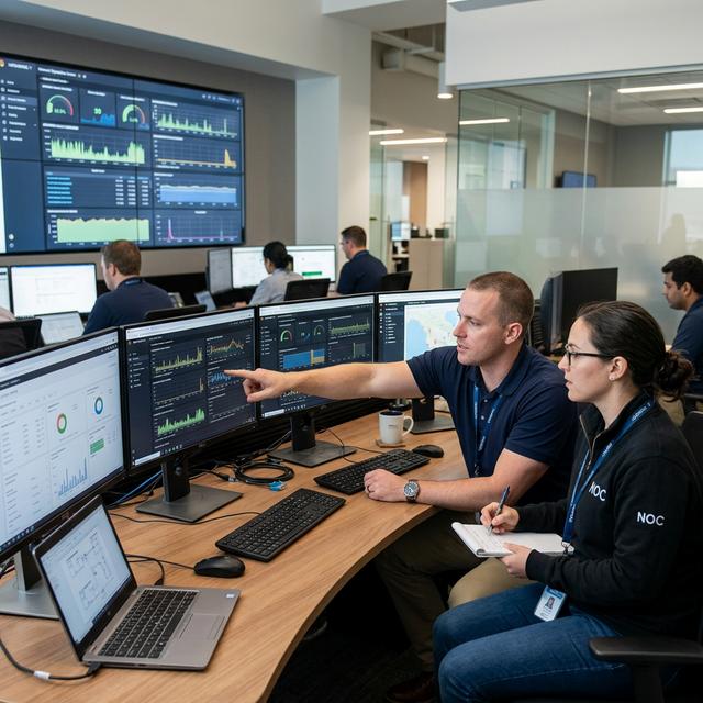
How to diagnose cold-query latency without fooling yourself
Begin with a controlled workload inventory. Select ten to twenty representative interactions: first dashboard open, date-filter change, high-cardinality drilldown, export, concurrent morning login and one exploratory query. Capture the actual SQL generated by the BI tool, the Redshift query identifiers where available, the timestamp and the user-visible completion time. Use sanitized test identities and protect any sensitive filter values.
For each interaction, collect the query start and end, queue and execution timing, relevant compilation or preparation evidence, bytes scanned or rows processed where available, result size, and the BI application’s own load time. Amazon Redshift system monitoring views, such as SYS_QUERY_HISTORY, and the platform’s monitoring tooling can help reconstruct warehouse behavior; check current column definitions before writing production monitoring SQL. Use the same dashboard version, data freshness and concurrency assumptions across comparison runs.
Compare three cohorts rather than one anecdote: genuinely new query shapes; repeated query shapes; and high-load executions. If a query is fast only on repeat, examine cache and compilation effects. If it is slow only during peak hours, investigate queuing and capacity. If the SQL is fast but the page remains slow, focus on the BI or application layer.
Do not benchmark by running one SQL statement twice and announcing a 70% improvement. That comparison changes several variables simultaneously, including compiled-code reuse and potentially result caching. Instead, record a distribution across many executions and show p50, p95 and worst-case values. Repeat at different load levels. Where feasible, disable or control relevant caches for diagnostic testing without changing production settings casually.
A practical measurement scorecard
Measure user experience: first meaningful chart render, full page load, filter response and export completion. Measure warehouse health: query queue time, preparation or compilation indicators, execution duration, throughput and concurrency. Measure data-product quality: freshness, metric correctness, error rate and permission failures. Measure economics: compute spend per reporting period or per thousand interactions, plus operational support effort.
Set thresholds based on the actual use case. An internal monthly board report may tolerate several seconds; an embedded customer-facing filter may not. Agree on an SLO before tuning. A reasonable scorecard might state that 95% of core executive interactions should complete within a chosen threshold during defined business hours, with explicit exclusions for exports and unusually large ad hoc analysis. The number should come from user research and baseline data, not a universal industry claim.
Keep the outcome separate from the mechanism. “Compilation time improved” is a technical result. “Executives can open their morning KPI dashboard within the agreed threshold during peak traffic” is the business result. The second is what should drive investment.

A diagnostic decision tree for BI leaders
If the first run is slow but repeats are fast, verify the Redshift version and investigate compilation and cache behavior. If both first and repeated runs are slow, inspect the query plan, table design, joins and amount of data processed. If only busy periods are slow, inspect queue time, concurrent ETL and capacity. If warehouse queries are fast but the report is slow, inspect generated-query count, connection overhead, result transfer and visual rendering. If only certain users are slow, investigate security predicates, row-level access, regional latency and their default filter scope.
If several problems coexist, prioritize the largest contribution to end-to-end latency. Improving a 100-millisecond step by 80% will not rescue a page waiting eight seconds on a different step. Maintain a ranked backlog with expected user impact, implementation effort, risk and evidence. This turns performance tuning from a sequence of guesses into an engineering program.
What to do with existing caching and pre-aggregation strategies
Do not dismantle proven materialized views, summary tables or application caches simply because compilation is faster. They solve different problems. A summary table reduces the amount of data processed; result caching avoids some repeated computation; compiled-code reuse reduces preparation overhead. Each has distinct correctness, freshness and operational trade-offs.
Reassess scheduled “warm-up queries” carefully. Some organizations run dashboards automatically before business hours to avoid cold starts. The new Redshift behavior may reduce the value of that practice for compilation-related delays. However, a warm-up could also populate result caches or trigger other work. Measure before retiring it, and document whether the practice has a freshness, cost or security consequence.
Similarly, pre-aggregation should be justified by query shape and latency requirements. A well-designed mart often improves maintainability and metric consistency as much as speed. Actiknow’s business intelligence and data modeling services describe a broader approach that includes source integration, modeling, visualization, publishing and refresh mechanisms, all of which affect the end-user experience.
A 30-day performance review that produces decisions
Week 1: establish the baseline
Identify the top five reports by business importance and the top ten slowest interactions by user impact. Capture page-level and SQL-level timings under realistic morning and off-peak load. Document Redshift cluster or Serverless configuration, maintenance patch, BI tool version, semantic-model design and refresh schedule. Confirm that monitoring does not expose sensitive query parameters to unnecessary audiences.
Week 2: classify the bottlenecks
Group interactions by dominant delay: preparation, execution, queueing, BI request fan-out, transfer or rendering. Review repeated versus novel query shapes. Produce a short evidence pack showing representative query IDs, timing distributions and a clear explanation of what is known versus inferred. Avoid attributing all improvements to the 2026 compilation release without a controlled comparison.
Week 3: implement the smallest high-value changes
Examples include removing redundant visuals, consolidating measures, improving a high-cost join, creating an appropriately refreshed aggregate, adjusting workload isolation or reducing the result payload. Make one change at a time where possible and use version-controlled SQL and dashboard definitions. Test that metric totals, security behavior and drilldowns remain correct.
Week 4: validate and operationalize
Repeat the baseline workload with equivalent data and concurrency. Compare p50 and p95 user-visible latency, queue time, execution time, error rate and compute consumption. Publish a decision memo: improvements achieved, unresolved bottlenecks, risks, next owners and monitoring thresholds. If no material improvement is measured, say so and stop the intervention rather than manufacturing a success story.

Questions to ask a vendor or internal platform team
Ask which latency component is currently largest, what proportion of real interactions use genuinely new query shapes, and whether the current Redshift patch includes the compilation optimization. Ask how the team controls for caching and concurrency in its benchmarks. Ask which dashboards have defined user-experience SLOs, how correctness is regression-tested after tuning, and who owns performance once the dashboard is live.
Be skeptical of isolated benchmark claims. AWS’s published results describe specific tests and environments. They are valuable evidence that the feature works, but your dashboard’s query mix, concurrency, data distribution and BI behavior determine the actual benefit. A credible performance proposal should show measurements from your environment, not only vendor marketing numbers.
Frequently asked questions
Why is my first Redshift query slower than the second?
Historically, a new query shape could incur one-time compilation overhead, while subsequent similar queries reused compiled code. Result caching and data caching can also make repeat runs faster. The 2026 composition optimization reduces the need to wait for compilation, but you should still separate these mechanisms in your measurements.
Did Amazon Redshift eliminate cold starts completely?
No. AWS reduced a specific compilation-related startup penalty. Connection establishment, queuing, scanning, joins, result transfer and application rendering can still produce slow first interactions. The phrase “cold start” is used for several different phenomena, so define which one you mean.
Does the 7x improvement apply to every dashboard?
No. AWS reported up to 7x faster new-query performance for relevant workloads. The benefit depends on how much time compilation previously consumed. Queries dominated by heavy execution or contention may show little visible improvement.
Do I need to enable the new Redshift feature?
AWS describes the optimization as automatically enabled, at no additional feature charge, on supported Redshift provisioned clusters and Serverless workgroups. Confirm your maintenance patch and deployment context against current AWS documentation before drawing conclusions from an older environment.
Should we stop using materialized views?
No. Materialized views and aggregates reduce execution work and can improve predictable performance. Faster query preparation does not eliminate expensive joins or scans. Evaluate each optimization against freshness requirements and measured workloads.
Will upgrading Redshift fix a slow Power BI or Tableau report?
It may reduce warehouse startup overhead, but it cannot fix redundant visual queries, inefficient semantic calculations, large result transfers or browser rendering. Profile the complete request path and prioritize the largest delay.
What is the best metric for an executive dashboard?
Use a user-visible metric such as p95 time to usable dashboard or filter response, supported by warehouse queue and execution diagnostics. Median query duration alone can hide painful peak-period experiences.
Is result caching the same as compiled-code caching?
No. Result caching can reuse an answer under applicable conditions. Compiled-code caching reuses prepared execution logic, but the query may still execute against data. Composition addresses the preparation path when optimized compiled code is not already available.
How can we test the feature without misleading benchmarks?
Use representative new and repeated query shapes, consistent data, comparable concurrency and multiple runs. Record end-to-end dashboard timing as well as warehouse components. Report distributions, not a single best run, and note any changes in cache or refresh state.
When should we consider more compute?
Only after evidence shows resource contention or execution capacity is the material bottleneck. More compute will not necessarily improve a dashboard dominated by network overhead, BI fan-out or unnecessary client-side rendering.
The bottom line
Redshift’s 2026 compilation optimization is good news for interactive analytics because it makes the first execution of unfamiliar SQL less likely to pay a large preparation penalty. But the next stage of dashboard performance improvement is more disciplined, not less: measure the complete user journey, distinguish cold compilation from cold data and busy compute, and optimize the largest verified bottleneck.
If your reporting team needs help separating warehouse performance from dashboard design issues, Actiknow can discuss a targeted performance review covering data integration, modeling, report behavior and measurable user experience. You can discuss a targeted performance review with Actiknow to scope a focused assessment rather than committing to a broad rebuild.
References and verification notes
Technical feature details: AWS’s March 18, 2026 announcement; AWS’s June 29, 2026 engineering explanation; Redshift cluster-version notes. Platform benchmarks cited here are AWS-reported, not Actiknow customer results. This article does not assert that Actiknow has implemented the specific 2026 Redshift feature for a named client.